Let's Learn LLL! Part 1

introduction

I’ve been wanting to write this for a LONG time (since about mid-2023 maybe), but I never got around to doing it. Somehow I’ve been super productive for the past few days though¹, so I thought I might as well cross one more thing off of my to-do list.

I’m splitting this introduction into the two parts: the first part (which you are reading now) will cover the mathematical background on lattices, while the second part will cover the applications of lattices in cryptography CTF challenges.

Anyways, since this is meant to be an introduction to lattices geared towards CTFers, I will not be very rigorous. Sorry.

prerequisites

I’m going to assume that you know at least the basics of linear algebra; if you aren’t, you can still read on, but you may not be able to fully comprehend everything.

lattices

Definition: A lattice that is spanned by basis vectors is defined as

The number is termed the dimension of the lattice. Generally we require that the basis vectors should be linearly independent, and thus . Furthermore, if , we say that the lattice is full-rank.

In other words, a lattice is the linear combinations of the basis vectors with integer coefficients.

Because a lattice is defined by vectors in , we can also represent a lattice as a matrix in , with the basis vectors forming the rows of the matrix.²

Here are some examples of lattices:

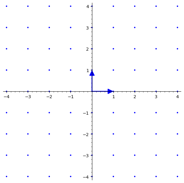
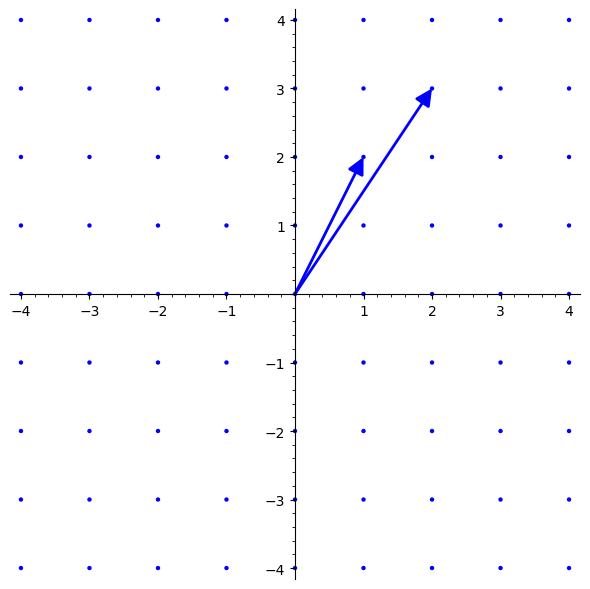
You might have noticed that these two different bases span the same lattice. In fact, there are infinitely many bases that span the same lattice. The following theorem shows why:

Theorem: Two bases span the same lattice if and only if there exists a unimodular matrix such that

A unimodular matrix is a integer matrix that has determinant . An important property of unimodular matrices is that their inverses are also unimodular. By the way, unimodular matrices of form a group denoted as .

Proof:

If: Since , the rows of are integer linear combinations of the rows of , and thus . Multiplying by on both sides, we have , and by a similar argument. Thus, we have that .

Only if: Since , the rows of are integer linear combinations of the rows of and vice versa. Thus, we have that and for integer matrices . From this we get and . Since we require the basis vectors of a lattice to be linearly independent, and . Since are integer matrices, their determinants must be integers too. Thus, we have that , and are unimodular.

fundamental domains and blichfeldt’s theorem

Definition: A fundamental domain of a lattice is any region such that the following holds true:

Informally, a fundamental domain is able to tile the span of the lattice basis by shifting by each lattice point. A specific fundamental domain of interest is the fundamental parallelepiped.

Definition: The fundamental parallelepiped of a lattice with basis vectors is defined as

In addition, we will also introduce the notion of the determinant for lattices.

Definition: The determinant of a lattice with is defined as

This quantity is also equal to the volume of the fundamental parallelepiped of treated as a -dimensional simplex.

Now we are ready to prove Blichfeldt’s theorem, a theorem that can be thought of as a continuous version of the pigeonhole principle.

Theorem (Blichfeldt’s theorem): For a lattice , if a set is such that then there exists such that .

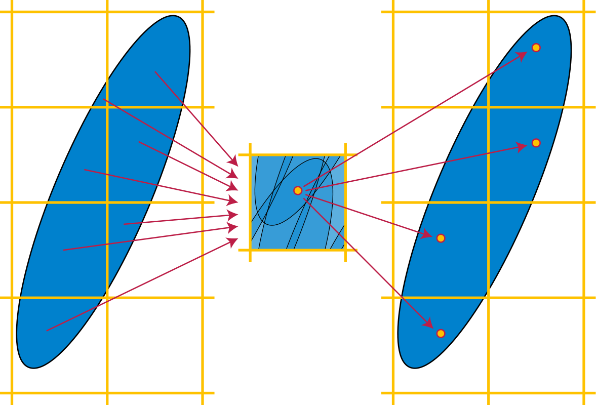
A formal proof is left as an exercise to the reader³, but a basic idea of the proof is that if we cut up space into shaped chunks, since , “by the pigeonhole principle” when we overlap all the chunks together there will always be multiple points in overlapping one another.

An important corollary of this theorem is Minkowski’s theorem.

Theorem (Minkowski’s theorem): Let be an -dimensional full-rank lattice. If a convex set is symmetric about the origin and , then there exists a point such that .

A convex subset means that for all and symmetric about the origin means that for all .

Proof: Let be a set that satisfies the conditions, and let . Then and by Blichfeldt’s theorem there exist such that . From the definition of we have that , so now consider . It is in due to the conditions of convexity and symmetricity we imposed, and it is equal to .

Minkowski’s theorem has an important application in bounding the length of the shortest vector, which we will discuss in greater length later.

tangent: fermat’s theorem (no, not that one)

Let’s take a short break from all the theorems and definitions, and look at a rather interesting application of Minkowski’s theorem.

In 1640, Fermat wrote in a letter to Mersenne that every prime can be expressed as with . This theorem is today an elementary theorem in number theory, and like a certain other theorem Fermat did not provide a proof of his statement.

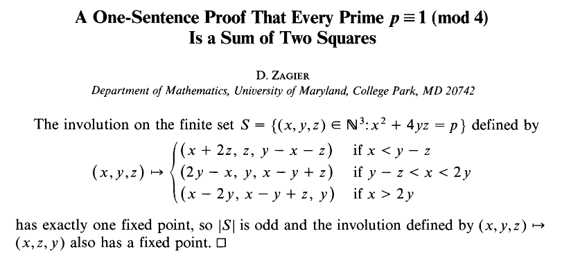
Fortunately, Euler “after much effort” found a proof based on infinite descent almost a hundred years later in the 1740s. Many other proofs followed, including Dedekind’s proofs(!) using Gaussian integers, and an incredible “one-sentence proof” that you might have seen online before.

There is also a (in my opinion) very nice proof using lattices and Minkowski’s theorem, shown below.

Proof: From Euler’s Criterion, we know that is a quadratic residue modulo , as . Let be an integer between and such that . Now consider the lattice spanned by basis

We can see that this is full rank and . Consider the set , that is, a circle centered at the origin with radius . Minkowski’s theorem says that since , there exist nonzero integers and such that . Reducing the expression modulo , we have that

and thus .

Pretty cool. This proof is non-constructive (meaning that it does not explicitly state how to obtain the two numbers that when squared sum to ), but we’ll see in the next part how we can obtain a solution.

successive minimums

Definition: the successive minimums for a lattice with is defined as

where represents the sphere with radius , that is,

What a mouthful. In simpler⁴ terms, the successive minimum is the length of the th shortest vector in the lattice, discounting vectors that are a linear combination of the short vectors. However, note that just because the vectors corresponding to the successive minimums are linearly independent, does not form a basis for the same lattice. For example,

has successive minimum vectors

where the last row is obtained from . However, , as .

Remember how I mentioned Minkowski’s theorem can bound the length of the shortest vector? Here it is.

Theorem: For a full rank -dimensional lattice , the following holds:

Note that is equal to the length of the shortest vector in . The proof will again be left as an exercise to the reader, as it is quite a simple application of Minkowski’s theorem.

lattice basis reduction

Earlier there was an example of two bases that span the same lattice; here they are again:

is, in a sense, a better basis for this lattice than , because its basis vectors are shorter than ’s. Lattice basis reduction is the process of transforming a lattice basis into a “better” one, where the basis vectors are hopefully shorter.

From here onwards, we will shift our attention from definitions to various lattice basis reduction algorithms, building up towards our final goal: the Lenstra-Lenstra-Lovász lattice basis reduction algorithm (LLL for short).

gram-schmidt orthogonalisation

As a refresher, the Gram-Schmidt orthogonalisation algorithm takes in vectors and returns orthogonal vectors defined as

where

For simplicity, I will be referring to and as the Gram-Schmidt vectors and Gram-Schmidt coefficients respectively. Note that we are not normalising the vectors here.

Here are some properties of the Gram-Schmidt vectors that are important: for forming the basis of lattice ,

Now, using the Gram-Schmidt vectors as a basis (get it), we can define the orthogonality defect of a basis to be

Since the determinant of the lattice is equal to the product of the Gram-Schmidt vectors, the orthogonality defect is essentially a measure of how not orthogonal a basis is. In the case where a basis is already orthogonal, the orthogonality defect is 1. It’s also easy to see that for all bases, .

Unfortunately, the Gram-Schmidt vectors are not always a basis of the lattice spanned by the original vectors. Let’s now look at actual lattice basis reduction algorithms, starting with a simple one for 2D lattices.

lagrange’s algorithm

Lagrange first formulated the notion of a reduced basis for a 2D lattice while researching quadratic forms in an article published in 1773.

Definition: A basis is said to be Lagrange-reduced (or simply reduced) if and only if and .

This definition is actually equivalent to the (perhaps simpler) definition with the condition that for all integer .

Proof: Consider . We have that for all integer ,

Since , it follows that and thus is bounded from below as follows:

As , we have that and the desired result is obtained upon taking square roots on both sides.

For the converse, we square, subtract , then divide by on both sides of the inequality to get

for all integer . By considering the cases where and , we can see that , and the desired result follows.

In fact, another equivalent definition is . As usual, the proof will be left as an exercise.

Geometrically, the Lagrange reduction constraints mean that must be shorter than , and the angle between them must be smaller than or greater than . The longer is compared to , the less orthogonal they must be.

Now, we will prove that and satisfying these conditions are indeed reduced.

Theorem: For and satisfying the Lagrange reduction constraints, they are the shortest vectors in the lattice spanned by them. That is, and .

Proof: We will first prove that is indeed a shortest vector, then prove that is a next shortest vector that forms a basis together with .

For an arbitrary nonzero vector in the lattice with not both zero. Consider .

Note that we only need to consider the case where . Completing the square,

Thus, for all vectors in the lattice, and so .

Now, let with not both zero be a vector that, together with , forms a basis for the lattice. Clearly . Let be integers such that and . We have that

Now, by the reverse triangle inequality,

Lagrange’s algorithm can be thought of as a 2D version of a variant of the Euclidean algorithm for finding the greatest common divisor of two numbers. Pseudocode (Python flavoured) for both algorithms are presented below:

# centered euclidean algorithm
def euclid(x, y):
    if abs(x) <= abs(y):
        x, y = y, x
    while y != 0:
        k = round(x/y)
        x, y = y, x - k*y
    return abs(n)

# lagrange's algorithm
def lagrange(x, y):
    if x.norm() < y.norm():
        x, y = y, x
    while x.norm() > y.norm():
        k = round((x*y)/y.norm()^2)
        x, y = y, x - k*y
    return x, y

Just for simplicity of proof later, we will assume that round() or rounds halves towards zero; that is, and . While the termination conditions for both algorithms differ, we can notice that both algorithms first ensure that the first parameter is larger than the second, and perform a “reduction” operation based on the rounded value of the “quotient” of both parameters.

To finish off this section, we will prove that Lagrange’s algorithm does indeed return a basis satisfying the Lagrange reduction conditions.

Proof: It is evident that in the loop spans the same lattice as . It is evident that Lagrange’s algorithm terminates; if the while loop were to not terminate, an infinite series of vectors in the lattice with strictly decreasing norm would exist, but we know that there is a smallest vector for every lattice.

Now we prove that the algorithm returns a reduced basis when it terminates. Call the vectors used in the last iteration of the loop and . We need to prove that and . The former is trivial by the termination of the algorithm, the latter can be proved by observing that

the lenstra-lenstra-lovász (LLL) algorithm

Lagrange’s algorithm, while guaranteed to return the most reduced basis in a lattice, only works for 2 dimensional lattices. The LLL algorithm, on the other hand, works for all lattices, but is not guaranteed to return the “most” reduced basis. We first need to define a new criteria for reducedness for a general lattice, since Lagrange reduction does not work well beyond 2 dimensions.

Definition: A basis is said to be -LLL-reduced if and only if the following two conditions hold.

1. For all , (size reduction)
2. For all , (Lovász condition)

where and are the Gram-Schmidt vectors and coefficients as mentioned previously, and .

The first condition can also be seen in the definition of Lagrange reduction, but the second is new and might be confusing at first glance. Unfortunately, I’ve not quite gained complete understanding of how these two conditions aid reduction and the algorithm itself, so I will link to a good overview of LLL by Cryptohack.⁵ The algorithm itself can be roughly described as repeatedly performing Gram-Schmidt orthogonalisation (rounding the s to ensure that the new vectors are still in the lattice) and swapping pairs of vectors by a heuristic represented by the Lovász condition.

We will be proving a claim about a bound on the length of the shortest vector in the basis returned by LLL.

Claim: for a LLL-reduced basis of the lattice , the shortest vector satisfies

Proof: By using the LLL-reduction conditions, we have that